Overview of article related to Rotation periods of asteroids

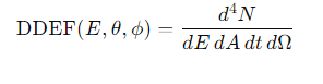
The Yarkovsky effect is a phenomenon that causes force to act on a rotating celestial body, such as an asteroid, due to the way it absorbs and re-emits sunlight as heat. The Yarkovsky effect depends on many physical and surface properties of the body such as diameter, albedo, density, obliquity, and rotation period.

The visual magnitude V of an asteroid is a measure of how bright it appears to an observer.  

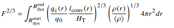
Heliocentric distance r is the distance between the object and the sun's center. 

H is the absolute magnitude of the asteroid,

Delta is range to the observer (in au), 

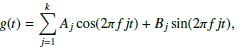
g(t) is a periodic function related to the asteroid shape in rotation, it is used to describe the repeating brightness variations (light curve) of an asteroid over time.

The phase function describes how brightness evolves with the phase angle(the Sun-asteroid-observer angle). The phase function is second-degree polynomial here.

To find g(t), fourier series has been used upto 10 order here.

If the shape of an asteroid is well-described by a tri-axial ellipsoid, the light-curve is expected to display two local maxima and two local minima. local maxima and local minima are the peaks and troughs of the asteroid's brightness variations over time. 

Source: https://arxiv.org/abs/2501.07189 

Read More

Key Points of article about new hydrogen-deficient white star

Scientists found 3 pre-white dwarfs (WDs) with helium-dominated atmospheres.

They calculated the effective temperature and surface gravity by comparing the He II line profiles of different stars.

Tübingen Model-Atmosphere Package tool was used for spectral analysis and to compute nonlocal thermodynamic equilibrium, plane-parallel, line-blanketed atmosphere models in radiative and hydrostatic equilibrium. It is based on the Accelerated Lambda Iteration method.

Kiel (Teff– log(g)) diagram was used to analyse the stars. The masses of stars were determined via comparison with evolutionary tracks using linear interpolation or Extrapolation and use of very late thermal pulse (VLTP)- a stage of evolution that occurs when a star re-ignites helium after leaving the Asymptotic Giant Branch (AGB) and still has a hydrogen-burning shell. By using these parameters, stellar radii was calculated by,

Luminosity was calculated by,

Gaia parallax distances can be used to derive masses, radii, and luminosities.

They used a spectral energy distribution (SED) graph that shows how much energy a star emits at different wavelengths. It's usually represented as luminosity per unit wavelength or frequency.

Source:

https://arxiv.org/html/2412.15984v1

Read More

Overview: Magnetic Field for Jupiter and Neptune Class exoplanets

Dynamo is the process by which a planetary magnetic field is generated through the movement of electrically conductive materials within the planet's interior. The dynamo region is identified based on the magnetic Reynolds number.

At the top of this region, the maximum magnetic field is 

 where 𝑞0 is the reference convective flux, ⟨𝜌⟩ is the average density,

𝐹 is an efficiency factor that accounts for all radially varying features of the dynamo region, and is calculated as 

where 𝐻T(𝑟) is the temperature length scale given by

 𝑃(𝑟) is the pressure, 𝑔(𝑟) the gravitational acceleration, and ∇adv the adiabatic, logarithmic gradient of temperature over pressure.

The convective flux 𝑞c is

𝑣conv the velocity of convective motions, and 𝛿 is the derivative of ln 𝜌 with respect to lnT.

Re mag is a non-dimensional quantity that measures the effects of convection against magnetic diffusion. 

As per study, for Jupiter and Neptune class planets, Magnetic field decay occurs because as planets age, they cool down and their luminosities and their convective flux become gradually weaker. Higher atmospheric envelope fractions cause more material available for convection, which yields stronger magnetic fields and extends the dynamo region.

 The field strength reduces for extremely irradiated planets because they have lower average density. The surface magnetic field decreases past the threshold value as orbital separation (distance between the exoplanet and its host star) further increases.

The magnetic fields could be observable in the radio wavelengths via auroral emission using ground based observations.

Jupiter-class planets have magnetic fields large enough to generate radiation whose peak frequency exceeds the Earth’s ionospheric cutoff. The same occurs for the Neptune-class planets  if they have  𝑀 > 15 𝑀⊕ and 𝑓env> 4%.

For hot jupiter class planets, atmospheric evaporation does not affect magnetic field generation. For hot Neptunes, atmospheric evaporation leads to greater mass loss and causes less material for convection, so they produce weaker magnetic fields. 

Source: https://arxiv.org/html/2411.00674v1

Read More

Key Points of Article about Measuring gravitational waves by graphene

Current detectors can only capture low-frequency gravitational waves.

By using graphene, higher frequency gravitational waves can be detected and size of detector also reduced. Here relative intensity varies when gravitational waves are measured.

As a gravitational wave propagates through a crystal lattice, it causes directional stretching and compression of the lattice, it causes shifts in the electronic energy band and density of energy states also changes.

Changes occur in graphene under gravitational wave,

Where,  yAB is the overlapping integral of the nearest neighbors, E is Graphene  energy

As per equations, gravitational waves alter the distances between carbon atoms in graphene, changing its lattice structure and causing a slight shift in the electron wave vectors. This affects the electronic transport behavior.

As gravitational wave radiation intensity hGW increases, the relative change in wave vector and wavelength increases.  

When the polarization direction of the gravitational wave is along the z-axis, the

the y-direction lattice of the photonic-like interferometer is stretched while the x-direction lattice is compressed. 

The change in Fermi energy is related to the shift of the energy band and the corresponding change in the density of energy states, which  affects gravitational waves on electrons in k-space. When the Fermi energy increases, the relative changes in the wave vector and wavelength decreases.

The relative intensity change (delta I/I )caused by arm length change in the photonic-like interferometer is about 2782 times larger than that in the laser interferometer because of the shorter electron wavelength.

Gravitational wave detection can be conducted by graphene at extremely low temperatures.

Source: https://arxiv.org/abs/2410.18711

Read More

Overview of Article about Magnetic helium-rich hot star found

 

Here the magnetic field was detected 200kG which is detected based on the zeeman effect. 

Zeeman effect: In zeeman effect, magnetic field distorts electron orbitals, which affects atomic energy levels and the transitions between them. This results in the splitting of atomic energy levels in a molecule, which in turn splits the spectral lines.

The splitting of a spectral line in the presence of a magnetic field is given by

Surface gravity is given by

Effective temperature is calculated based on 

The radial velocity is calculated using the Doppler effect equation:

Δλ = observed wavelength shift .

λ0 = rest wavelength of the spectral line

Galactic space velocities for the confirmed magnetic He-sdOs are calculated from their radial velocity.

Magnetic fields can cause dark or bright spots on a star’s surface, resulting in variations in brightness as the star rotates

Here the Hertzsprung-Russell diagram is used to compare the magnetic He-sdO stars with non-magnetic hot subdwarfs and other stars based on their temperature, luminosity, and mass.  

In the article, the mass of the magnetic He-sdO stars is estimated based on their location relative to the helium main sequence. The mass is interpolated from their position on the diagram.

When stars plot the same region of the H-R diagram, it indicates that they likely formed through a specific and same process.

Reference: https://arxiv.org/abs/2410.02737 

Read More

Summary of Article about Mercury’s plasma environment

The instruments designed to measure ions in Mercury’s plasma environment are: 

Mass Spectrum Analyzer (MSA), Mass Ion Analyzer (MIA), and Mass Electron Analyzer (MEA).

• Mass Spectrum Analyzer: This instrument has a spherical top-hat analyzer for energy analysis and a Time-Of-Flight (TOF) chamber for mass analysis.
• For ions passing through the top-hat analyzer, the energy-to-charge ratio is:

• This energy allows the MSA to filter ions with specific energies before they enter the Time Of Flight chamber. TOF analyzer measures the time t it takes for ions to travel a fixed distance d after they pass through the top-hat analyzer. From the TOF data, the ion’s velocity can be calculated. Then the mass-to-charge ratio m/q is calculated.

• The MSA uses a reflectron TOF system, which improves the mass resolution by reflecting ions back and forth within the TOF analyzer. If there are small differences in ion velocities, more accurate m/q can be measured.

Differential Directional Energy Flux (DDEF) of the ions and electrons is measured by MSA, MIA and MEA.

• N is the number of particles,
• E is the particle energy,
• A is the detector area,
• T is time, Ω is the solid angle,
• Θ and ϕ represent the direction of travel of the particles in spherical coordinates.

Magnetospheric regions and ion composition:

• The low latitude boundary layer(LLBL) is a region where magnetosheath and magnetospheric plasmas are mixed along the magnetospheric side of the low-latitude. There is presence of an energy dispersion( how particles with different energies spread out as they travel through a magnetic field of the ions). This dispersion extends from ~20 keV e−1 in the outer part of the flank down to 10s of eVs per e in the inner part.

• Kelvin-Helmholtz Instability occurs at the interface between two plasma flows with different velocities, such as between the solar wind (a stream of charged particles from the Sun) and a planetary magnetosphere or at the boundary of different plasma regions.

• In study, H+  trajectories were computed using a modified Luhmann–Friesen model for the magnetic field combined with convection pattern for the electric field. The full equation of motion was integrated  using a fourth-order Runge–Kutta technique.

• The plasmas sheet horns: In this region, there is presence of ~1 keV e−1 ions in the near-tail central plasma sheet extending to the higher latitudes.

• The flyby provided direct evidence of Mercury’s ring current. It is a circulating flow of charged particles around the planet, having energetic hydrogen ions (H⁺) and heavier ions like oxygen (O⁺)
• The ion observations highlight the presence of cold ions (≤50 eV e−1 ) and energetic ions (up to 38 keV e−1 ) in the environment. Energetic electrons up to 10 keV e−1 were also observed in the deep magnetosphere. 

https://www.nature.com/articles/s42005-024-01766-8

Read More